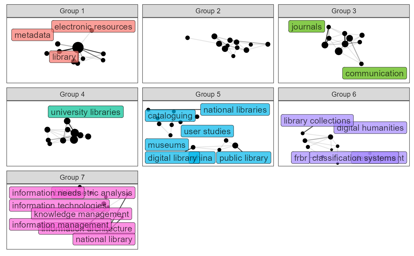
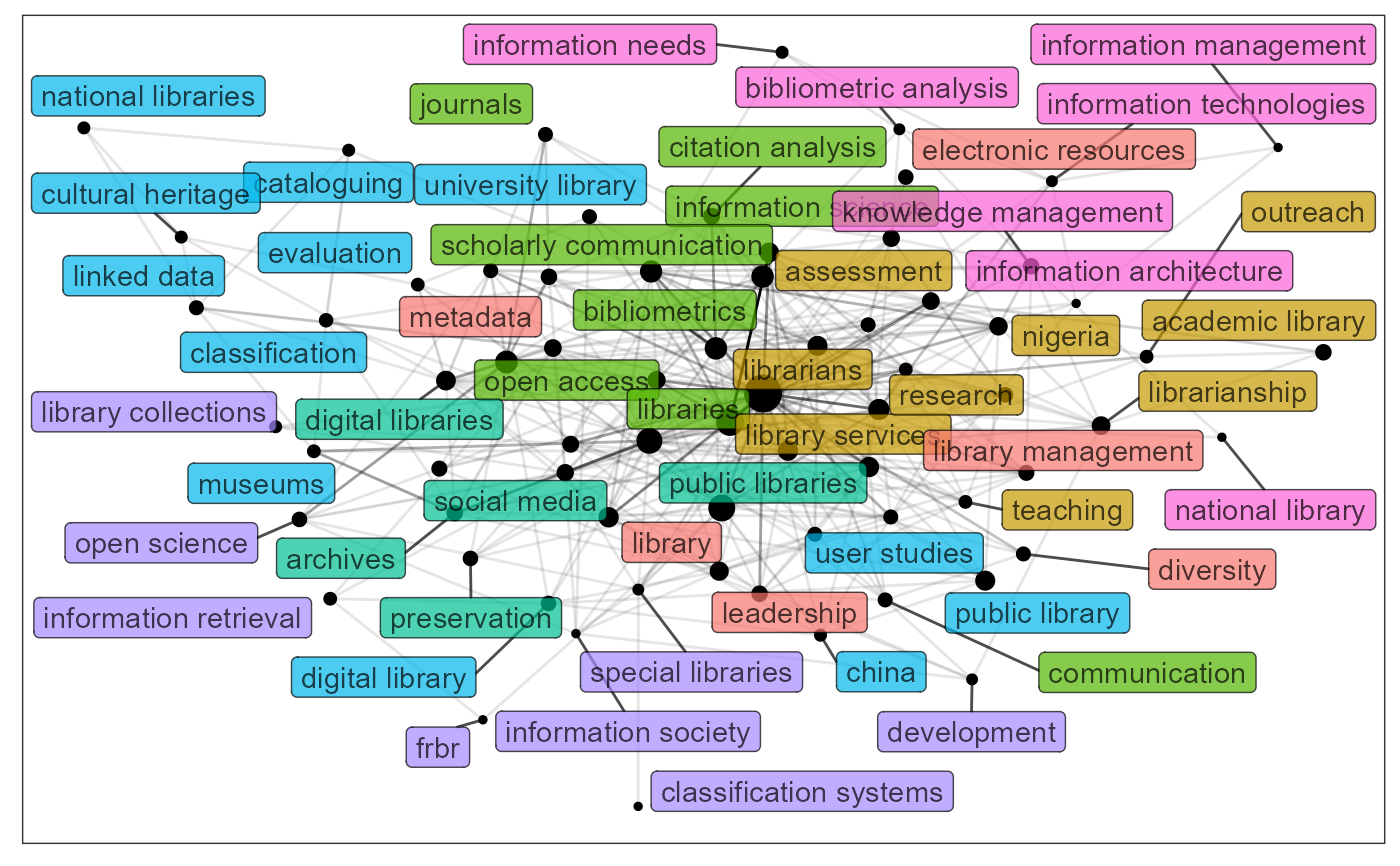
Visualization of grouped keyword co-occurrence network

Visualization of network-based keyword clustering, with frequency and co-occurrence information attached.

keyword_vis(tibble_graph, facet = TRUE, max_nodes = 10, alpha = 0.7)

Arguments

tibble_graph

A tbl_graph output by keyword_group.

facet

Whether the figure should use facet or not.

max_nodes

The maximum number of nodes displayed in each group.

alpha

The transparency of label. Must lie between 0 and 1. Default uses 0.7.

Value

An object yielded by ggraph

Details

When facet == TRUE,the function returns a faceted figure with limited number of nodes (adjuseted by max_nodes parameter).When facet == FALSE,all the nodes would be displayed in one network.Colors are used to specify the groups, the size of nodes is proportional to the keyword frequency, while the alpha of edges is proportional to the co-occurrence relationship between keywords.

See also

ggraph

Examples

library(akc)
# \donttest{
bibli_data_table %>%
  keyword_clean(id = "id",keyword = "keyword") %>%
  keyword_group(id = "id",keyword = "keyword") %>%
  keyword_vis()
#> Warning: ggrepel: 4 unlabeled data points (too many overlaps). Consider increasing max.overlaps
#> Warning: ggrepel: 8 unlabeled data points (too many overlaps). Consider increasing max.overlaps
#> Warning: ggrepel: 11 unlabeled data points (too many overlaps). Consider increasing max.overlaps
#> Warning: ggrepel: 4 unlabeled data points (too many overlaps). Consider increasing max.overlaps


# without facet
bibli_data_table %>%
  keyword_clean(id = "id",keyword = "keyword") %>%
  keyword_group(id = "id",keyword = "keyword") %>%
  keyword_vis(facet = FALSE)
#> Warning: ggrepel: 3 unlabeled data points (too many overlaps). Consider increasing max.overlaps


# }