Tutorial for knowledge classification from raw text

Huang Tian-Yuan (Hope)

This tutorial gives an example of how to use akc package to carry out automatic knowledge classification based on raw text. First, load the packages we need.

library(akc)
library(dplyr)
#> 
#> Attaching package: 'dplyr'
#> The following objects are masked from 'package:stats':
#> 
#>     filter, lag
#> The following objects are masked from 'package:base':
#> 
#>     intersect, setdiff, setequal, union

Inspect the data

In the dataset, we have the ID, title, keyword and abstract of documents. We are going to use the keyword as the dictionary to extract keywords from the abstract.

bibli_data_table
#> # A tibble: 1,448 × 4
#>       id title                                                   keyword abstr…¹
#>    <int> <chr>                                                   <chr>   <chr>  
#>  1     1 Keeping the doors open in an age of austerity? Qualita… Auster… "Engli…
#>  2     2 Comparison of Slovenian and Korean library laws         Compar… "This …
#>  3     3 Analysis of the factors affecting volunteering, satisf… Contin… "This …
#>  4     4 Redefining Library and Information Science education a… Curric… "The p…
#>  5     5 Can in-house use data of print collections shed new li… Check-… "Libra…
#>  6     6 Practices of community representatives in exploiting i… Commun… "The p…
#>  7     7 Exploring Becoming, Doing, and Relating within the inf… Librar… "Profe…
#>  8     8 Predictors of burnout in public library employees       Emotio… "Work …
#>  9     9 The Roma and documentary film: Considerations for coll… Academ… "This …
#> 10    10 Mediation effect of knowledge management on the relati… Job pe… "This …
#> # … with 1,438 more rows, and abbreviated variable name ¹​abstract

Get the dictionary from keyword field

keyword_clean is designed to split the keywords and removed pure numbers and contents in the parentheses. All letters would be converted to lower case. Details see the help of keyword_clean, use “?keyword_clean”. After cleaning, we’ll use these keywords to establish a dictionary.

bibli_data_table %>%
  keyword_clean() %>%
  pull(keyword) %>%
  make_dict() -> my_dict

Extract keywords from abstract

Using keyword_extract to extract keywords from the abstract. Here, we also exclude the stop words using the “stopword” parameter.

# get stop words from `tidytext` package
tidytext::stop_words %>%
    pull(word) %>%
    unique() -> my_stopword
  
bibli_data_table %>%
    keyword_extract(id = "id",text = "abstract",
    dict = my_dict,stopword = my_stopword) -> extracted_keywords
#> Joining, by = "keyword"

Merge keywords with same meanings

While this process has consider lots of factors, such as stemming, lemmatizing, etc. Here I’ll provide a easy implementation. For advanced usage, use “?keyword_merge” to find out.

extracted_keywords %>% 
  keyword_merge() -> merged_keywords

Divide keywords into groups (automatic classification)

This process will construct a keyword co-occurrence network and use community detection to group the keywords automatically. You can use “top” or “min_freq” to control how many keywords should be included in the network. “top” means how many keywords with largest frequency should be included. “min_freq” means the included keywords should emerge at least how many times. Default uses top = 200 and min_freq = 1.

merged_keywords %>% 
  keyword_group() -> grouped_keywords

Get the grouped table

Getting the result as a table could be easy by:

grouped_keywords %>% 
  as_tibble()
#> # A tibble: 203 × 3
#>    name         freq group
#>    <chr>       <int> <int>
#>  1 library      1583     1
#>  2 information   583     1
#>  3 data          437     1
#>  4 librarians    398     1
#>  5 academic      351     2
#>  6 design        338     1
#>  7 analysis      301     1
#>  8 development   254     2
#>  9 collection    283     2
#> 10 research      589     1
#> # … with 193 more rows

If you only wants the top keywords to be displayed, keyword_table provides another relatively formal table:

grouped_keywords %>% 
  keyword_table()
#> # A tibble: 2 × 2
#>   Group `Keywords (TOP 10)`                                                     
#>   <int> <chr>                                                                   
#> 1     1 library (1583); research (589); information (583); data (437); universi…
#> 2     2 academic (351); collection (283); development (254); academic libraries…

In such implementation, only two groups are found. You can specify the number of top keywords using “top” parameter.

Visualization of the network

Currently, keyword_vis,keyword_network and keyword_cloud could all be used to draw plots for the network, but in differnt forms. Let’s try to draw a word cloud first:

grouped_keywords %>% 
  keyword_cloud()

To get the word cloud of one group,use:

grouped_keywords %>% 
  keyword_cloud(group_no = 1)

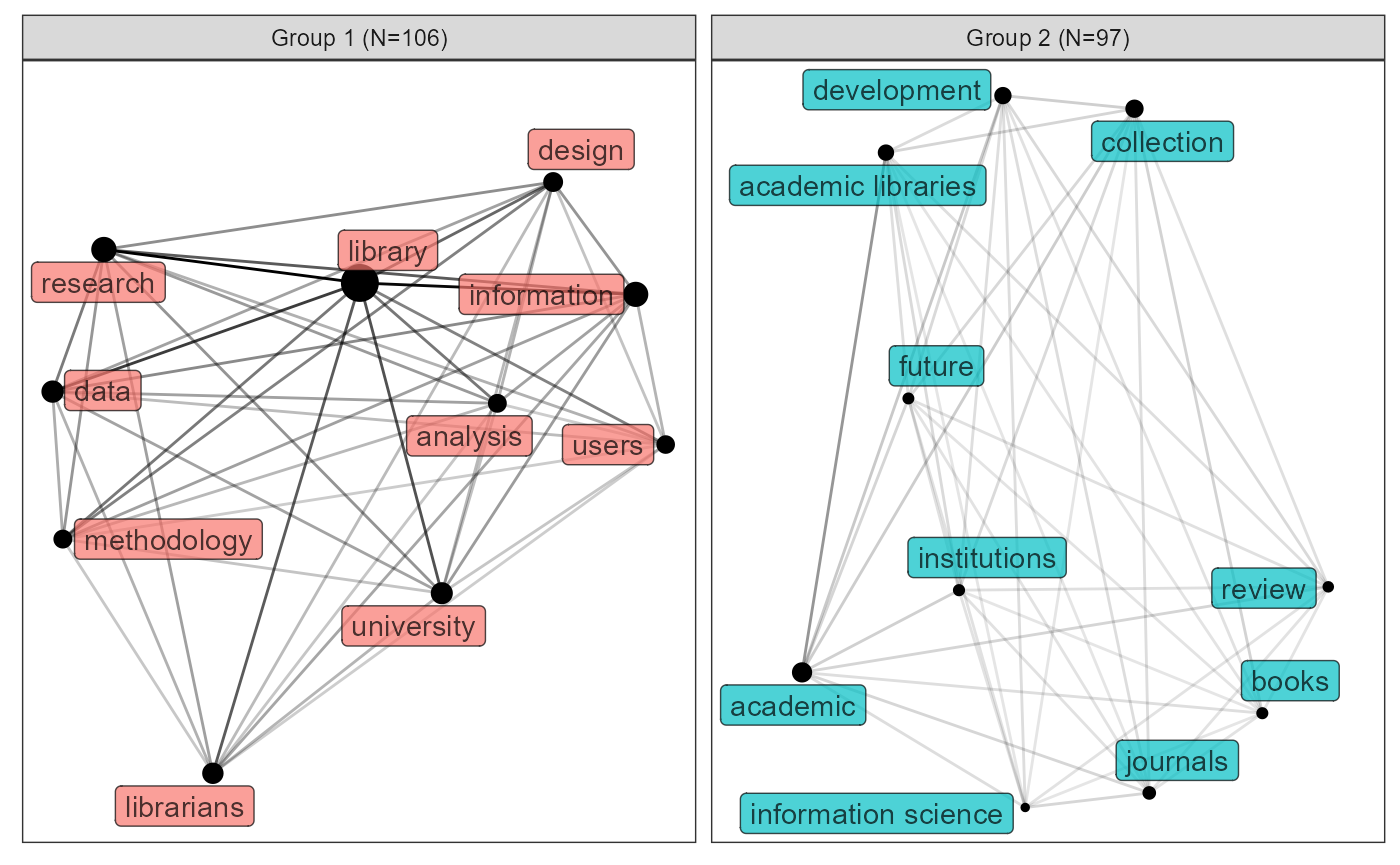
If you want to draw a network, use keyword_network:

grouped_keywords %>% 
  keyword_network()
#> Joining, by = c("name", "freq", "group")

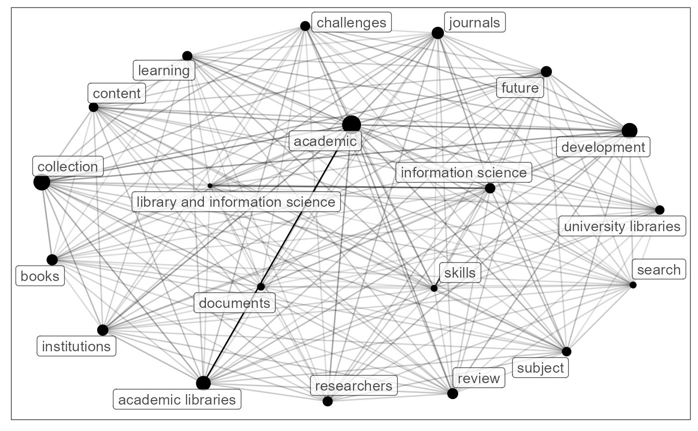
In the plot, “N=106” means altogether there are 106 keywords in the group, though only the top 10 by frequency are showed in the graph. If you only want to visualize the second group and display 20 nodes, try:

grouped_keywords %>% 
  keyword_network(group_no = 2,max_nodes = 20)

Have fun playing with akc!